Diabetes Data Diving
Analyzing diabetes patient data
Project maintained by NilaiVemula Hosted on GitHub Pages — Theme by mattgraham
MATH 2820L Final Project: Diabetes Data Diving
By Nilai Vemula, Anvitha Kosuraju, and Sithara Samudrala
Nilai Vemula did the modeling work (linear regression and random forest). Anvitha Kosuraju did the introduction and the exploratory data analysis for polyuria, polydipsia, sudden weight loss, and partial paresis variables. Sithara Samudrala completed the correlation matrix, chi-square feature selection process, exploratory data analysis for the age and gender variables, and the conclusion.
- Introduction
- Data
- Model
- Conclusion
Introduction
The data we are analyzing were collected using direct questionnaires from patients from the Sylhet Diabetes Hospital that were located in Sylhet, Bangladesh. We found this data through the UCI Machine Learning Repository. Our data is collected from 520 patients from this hospital. The data provides information that points to possible correlations between having diabetes and other factors. These other factors include age, sex, polyuria, polydipsia, sudden weight loss, weakness, polyphagia, genital thrush, visual blurring, itching, irritability, delayed healing, partial paresis, muscle stiffness, alopecia, and obesity. Out of these variables, we had one ordinal variable, which was age. All of the other variables were categorical with either a “yes” or “no” answer. The response variable was “Class”, which could either be “positive” or “negative” for diabetes. All of the answers from this questionnaire were approved by a doctor to make it reliable.
Through this project, we want to understand these possible and common risk factors that are tied to diabetes and to understand any patterns that occur between having diabetes and the presence of risk factors such as old age, obesity, polyuria, polydipsia, and other factors mentioned within the dataset. The main problem that we are trying to tackle is to see the patterns that occur within the data and decipher these patterns. We want to find the patterns that occur with the factors that are presented within the data and the presence of Diabetes within the individual. By finding these patterns, we can flag individuals with similar factors that might indicate that the individual has a high chance of developing diabetes. One of the most important things with overcoming diabetes is early diagnosis, so by finding these patterns that occur between certain factors and having diabetes, we can help find these flags that can lead to an early diagnosis.
In conclusion, our main goals were to analyze the various data that were included to make important conclusions about diabetes and related medical conditions. We also wanted to build a predictive model to be able to accurately determine if a specific patient has diabetes given their medical data, history, and symptoms. Additionally, we want to be able to determine which factors out of the variables in our data are the best predictors for if a specific patient will be diagnosed with diabetes or not.
Data
In the dataset, out of the 520 patients, 320 of the patients were diagnosed with Diabetes and 200 of the patients were not diagnosed with Diabetes. This is important to know, so we can see the factors that predominantly occurred with the 320 patients that were diagnosed versus 200 patients that were not diagnosed with diabetes.
Correlation Matrix
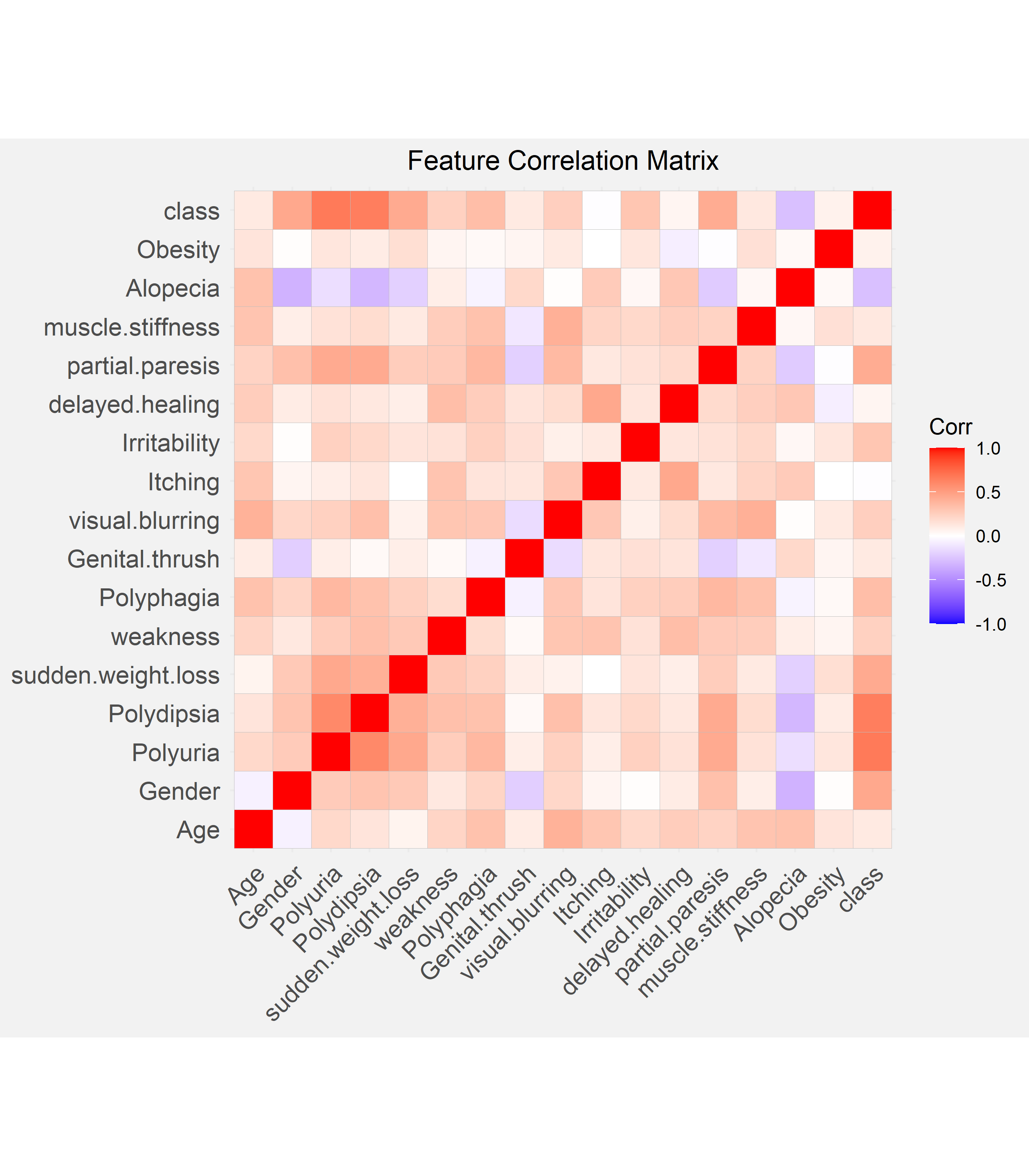
We calculated the Pearson correlation coefficient for each combination of features and visualized this in the form of a correlation matrix. In the matrix, the darker squares signify a greater correlation. The response variable, class, or the diagnosis of diabetes is most strongly and positively associated with polyuria and polydipsia, out of all the features. On top of this, polyuria also has a positive and moderately strong association with polydipsia.
Feature Selection
Chi-square feature selection was used as our method for selecting some of our 15 categorical predictor variables for further analysis. We aimed to select the top features that are most dependent on the response variable, class, or the diagnosis of diabetes. Since the Chi-square feature selection method tests the independence between two variables, we can compare the calculated chi-squared test statistics to determine which features are most dependent on class. Hence, if the chi-squared test statistic is greater, this is more likely to indicate that the feature and class are not independent or in other words, dependent.
| Feature | $\chi^2$ Test Statistic |
|---|---|
| Polyuria | 227.9 |
| Polydipsia | 216.2 |
| Gender | 103.1 |
| Sudden Weight Loss | 97.3 |
| Partial Paresis | 95.4 |
| Polyphagia | 59.6 |
| Irritability | 45.2 |
| Alopecia | 36.1 |
| Visual Blurring | 31.8 |
| Weakness | 29.8 |
Selected Features
We chose the variables with the highest chi-square values (Polyuria, Polydipsia, Gender, Sudden Weight Loss, and Partial Paresis) along with Age to investigate further.
When analyzing the various features we selected, we first came to an initial hypothesis as a group. We then created bar charts to provide an analysis of the specific variable and how this affects the possibility of diagnosis for diabetes. Then, we came to a conclusion based on our analysis of the bar chart. Our conclusion was based on if our bar chart supported or contradict the initial hypothesis, and what our bar chart indicated was the relationship between the variable and the possible diagnosis for diabetes.
Age
Initial Hypothesis
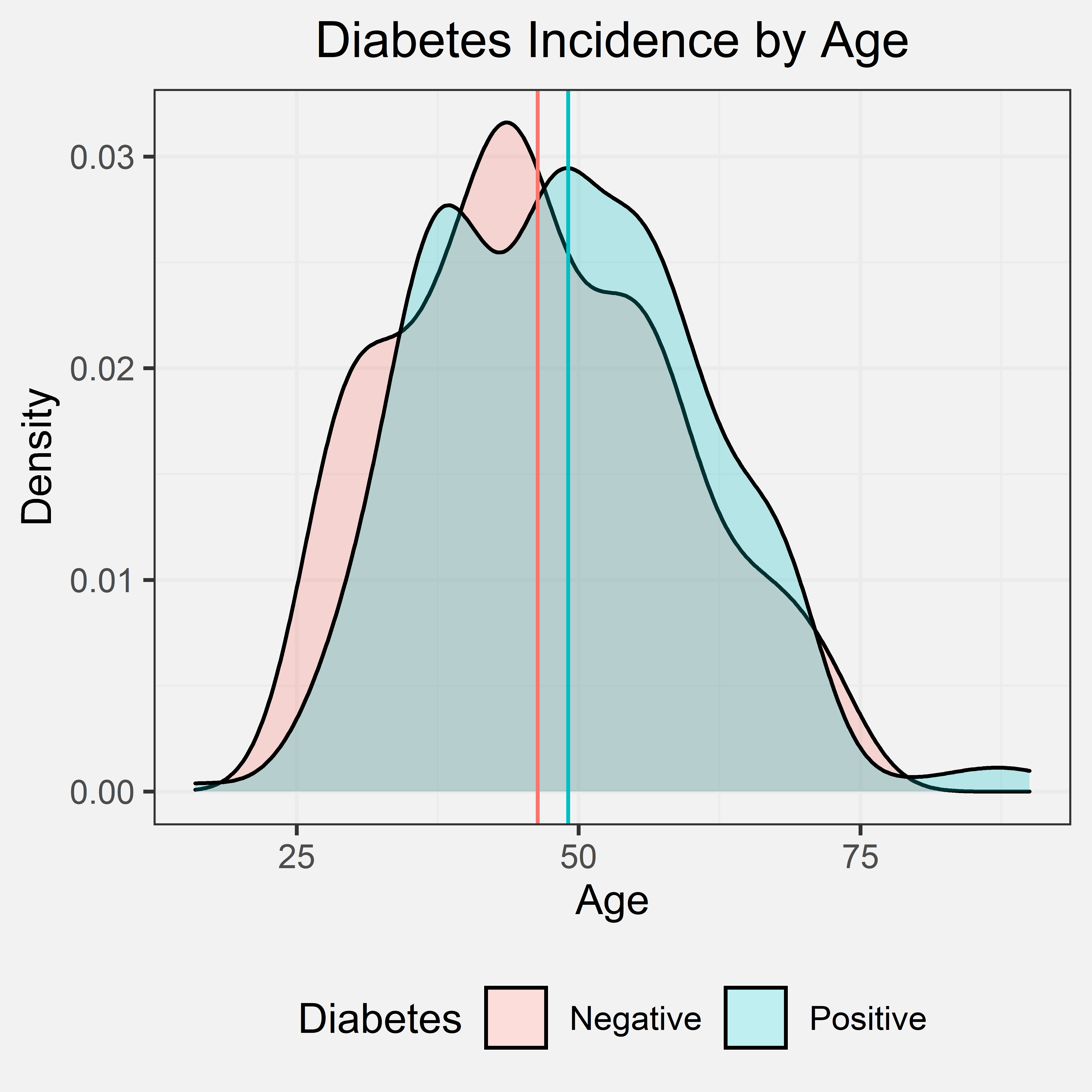
Our initial hypothesis was that if the patient was older, the patient has a higher chance of being diagnosed with diabetes. This initial hypothesis was primarily based on our prior experience and knowledge. Most of the individuals that we personally know that are diagnosed with diabetes were diagnosed later in life, but we did consider how there are two types of diabetes and the onset of these two types. Type I typically is diagnosed in children and teens and Type II is typically diagnosed in adulthood. Given that Type II diabetes is notably more prevalent than Type I, we still expect the data to show a positive correlation between age and diabetes diagnosis though the data does not distinguish between either type of diabetes. Out of the 520 patients that were interviewed, the ages ranged from 16 to 90. The mean age of the patients with diabetes was 49.07, and the mean age of the patients without diabetes was 46.36.
Density Plot
Conclusion
From the density graph and the indicated mean ages of patients with and without diabetes, we can tell that there is only a slightly higher average age for patients with diabetes and patients without diabetes. This shows that age is likely not a significant factor for diabetes. However, the data was collected at a diabetes hospital and did not account for diabetes type as a potential confounding variable. We cannot make any significant conclusions, but either way, the density graph does not support our initial hypothesis.
Gender
Initial Hypothesis
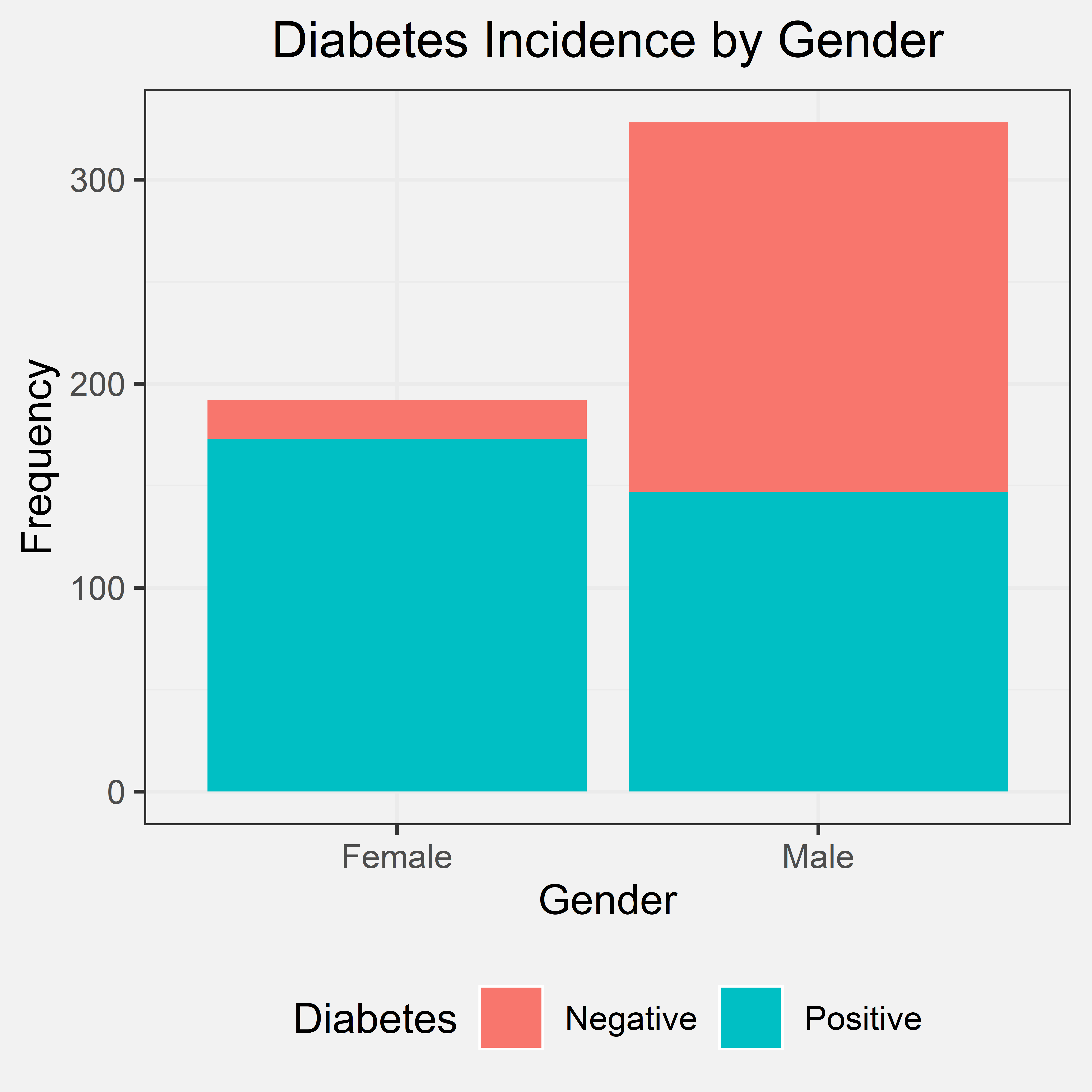
Gender was only characterized by two distinct sexes: male and female. Our initial hypothesis was that gender would have not effect on chances of diabetes in which the primary basis for this hypothesis was prior knowledge. Therefore, we expect to see the proportion of diabetes to be fairly even between the two genders. Out of 520 patients interviewed, 328 were male and 192 were female.
Bar Chart
Conclusion
From the bar chart, the frequency of male patients was far greater than the frequency of female patients. In this dataset, the majority of the patients with diabetes are female overall, despite how the frequency of male patients outnumber female patients in the dataset in total. Within the female patients, an overwhelming majority of the females were diagnosed with diabetes unlike and in comparison to the male patients in the dataset. The bar chart does not support our initial hypothesis, though it seems that female patients have a higher risk for diabetes with gender as a possible indicator for diabetes as a whole.
Polyuria
Initial Hypothesis
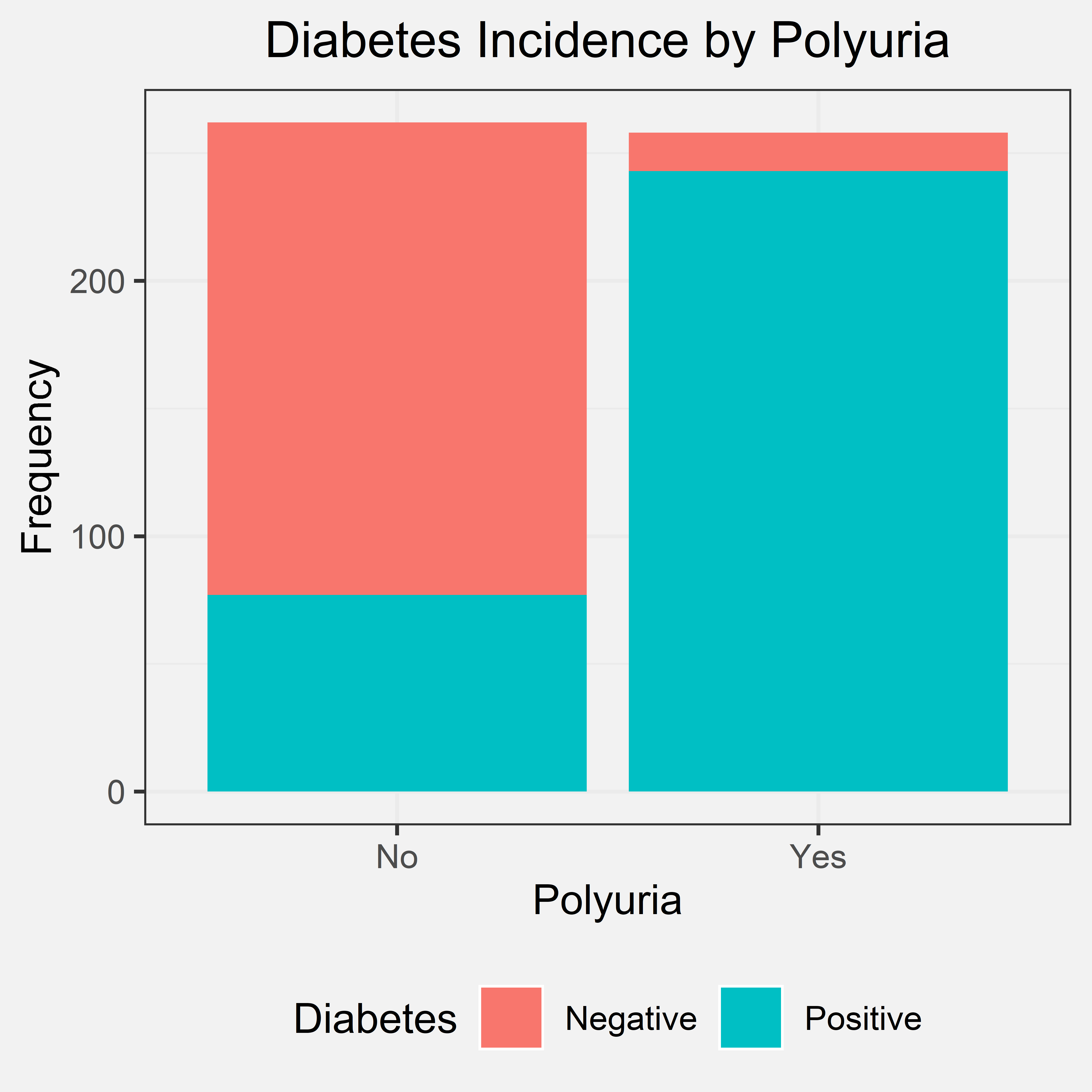
Polyuria is the production of abnormally large volumes of dilute urine. Our initial hypothesis was that if the patient experienced polyuria, they have a higher chance of being diagnosed with diabetes. We came to this initial hypothesis through some research and prior knowledge. If an individual has diabetes, they tend to have higher blood sugar levels, and their kidney will try to filter out their high blood sugar levels. This produces a lot of excess urine, leading to polyuria. Out of the 520 patients that were interviewed, 258 had polyuria and 262 did not have polyuria.
Bar Chart
Conclusion
From the bar chart, we can tell that a great number of individuals who were diagnosed with diabetes experienced polyuria. A few patients that were not diagnosed with diabetes also experienced polyuria, but there was a greater difference in the frequencies in the two situations. Due to this great difference, we can conclude that nearly all patients with polyuria have diabetes. Therefore, if a patient experiences polyuria, they have a higher chance of being diagnosed with diabetes. This shows us that a possible predictor/indicator for whether an individual has diabetes should be polyuria. Our bar chart also agreed with our initial hypothesis.
Polydipsia
Initial Hypothesis
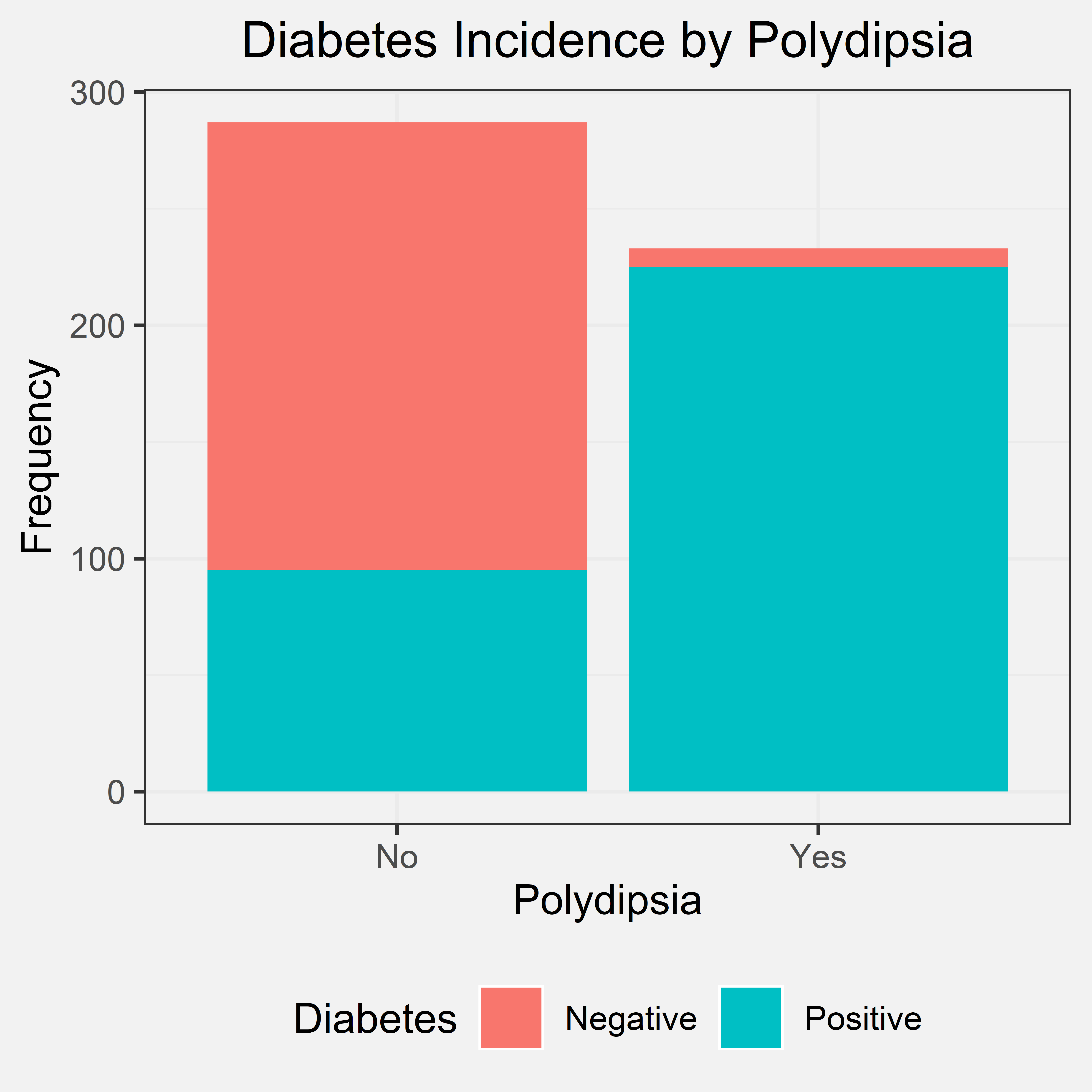
Polydipsia is another term for abnormally excessive thirst. Our initial hypothesis for polydipsia was that if an individual experienced polydipsia, then they have a much higher chance of being diagnosed with diabetes. We came to this hypothesis through prior knowledge. Excessive urine production or polyuria can lead to excessive thirst or polydipsia. When the body produces these high levels of sugar within the body, the body will produce increased levels of urine to get rid of excess sugar. Due to this increased level of urine production, it can lead to dehydration within the body leading to polydipsia. Out of the 520 patients that were interviewed, 233 said “yes” to experiencing polydipsia, and 287 said “no”.
Bar Chart
Conclusion
By looking at the bar chart, we can see that nearly all patients that experienced polydipsia were diagnosed with diabetes. Some individuals that said “no”, were also diagnosed with diabetes. However, almost every individual that said “yes” to polydipsia was later diagnosed with diabetes. We concluded that nearly all patients with polydipsia have diabetes. Therefore, if a patient experiences polydipsia, they have a higher chance of being diagnosed with diabetes. This conclusion and the bar chart support our initial hypothesis because a patient having polydipsia is an important indicator that they might also have a diagnosis. Therefore, polydipsia can be used as a predictor/indicator for diabetes due to these patterns.
Sudden Weight Loss
Initial Hypothesis
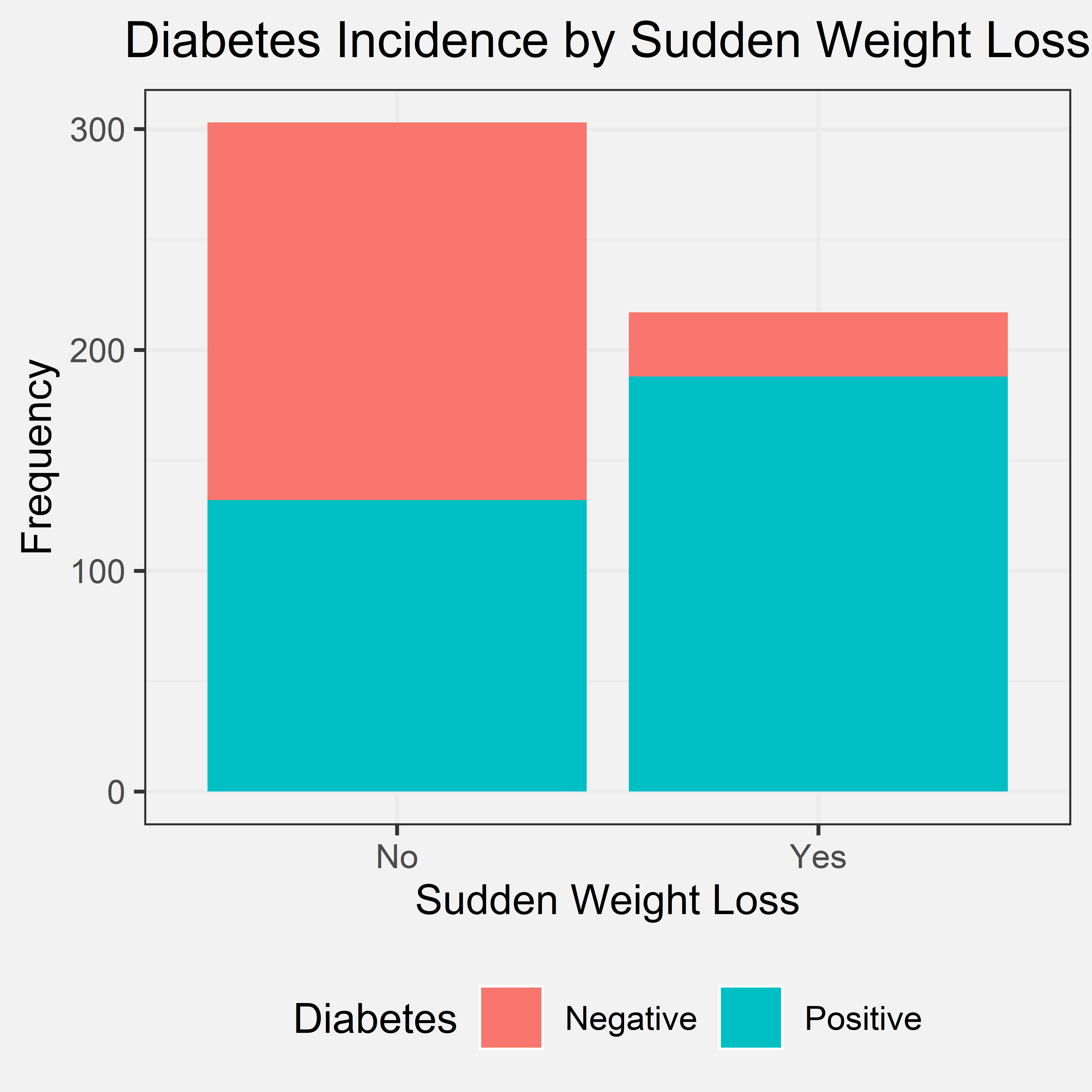
Our initial hypothesis for sudden weight loss was that if an individual had recently experienced sudden weight loss, then they have a much higher chance of being diagnosed with diabetes. We came to this hypothesis due to prior knowledge. Insufficient insulin prevents the body from getting glucose from the blood into the body’s cells to use as energy. Due to the body not having this instant source of energy, the body must instead use stored fat within the body as a way to get energy. The body starts to burn fat and muscle for energy, causing a reduction in overall body weight. Therefore, we believe that if a patient experiences sudden weight loss, then they have a high chance of being diagnosed with diabetes. Out of the 520 patients that were interviewed, 217 experienced sudden weight loss, and 303 did not.
Bar Chart
Conclusion
From the bar chart, we can see that a loss of individuals that said yes to experiencing sudden weight loss also was diagnosed with diabetes. There were a few who experienced sudden weight loss and were still not diagnosed with diabetes. Several individuals did not experience sudden weight loss and were still diagnosed with diabetes. Even though, sudden weight loss has a smaller amount of difference between the two values compared to polydipsia and polyuria; however, there is still a significant difference. Therefore, we concluded that if a patient has had sudden weight loss, it is very likely that they have diabetes, but the converse is not true. We did not include the second part within the initial hypothesis because we did not think about the pattern for the converse. However, the first part of our conclusion agrees with our initial hypothesis. Therefore, sudden weight loss can be used as a predictor/indicator of whether the patient will have diabetes or not.
Partial Paresis
Initial Hypothesis
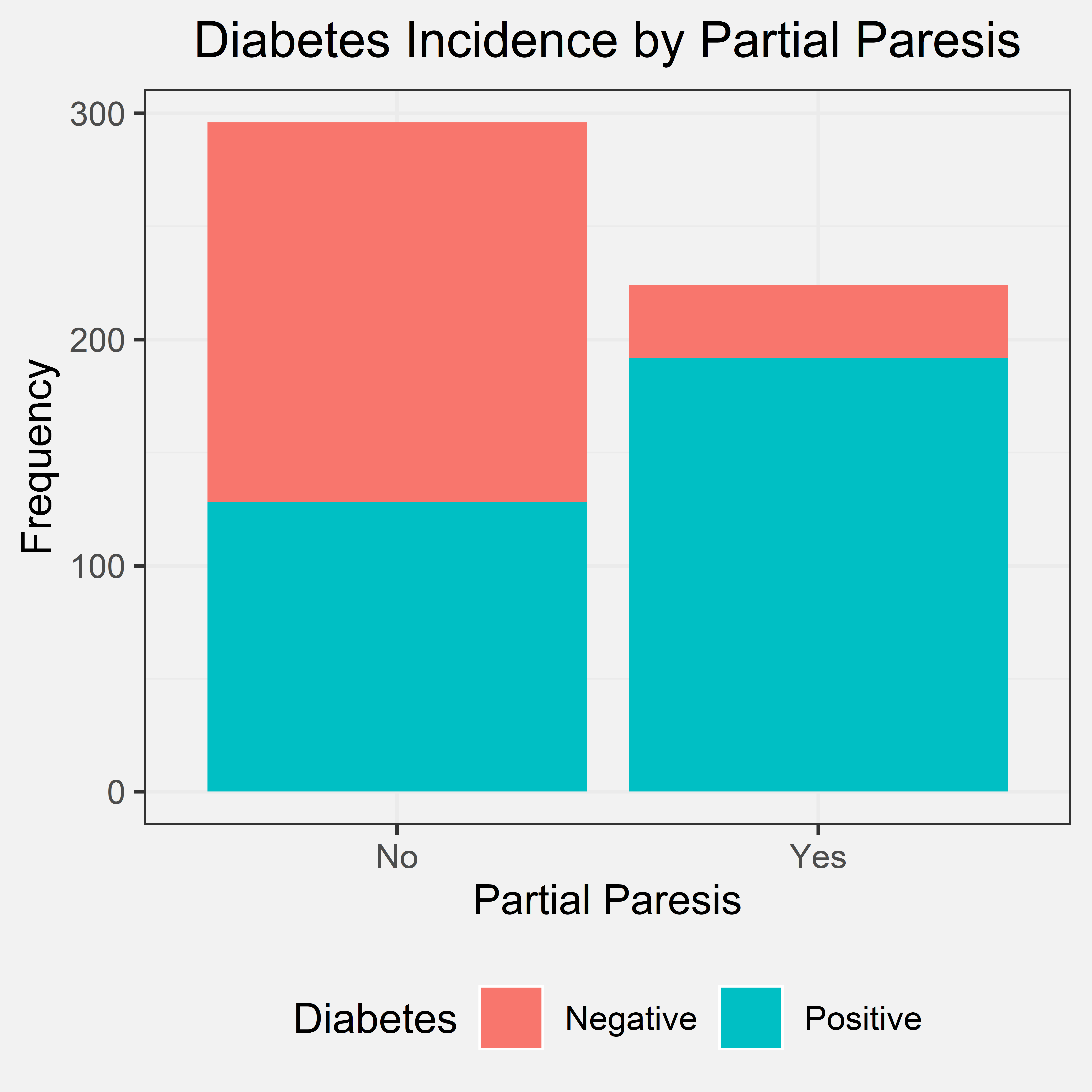
Paresis is a condition typifies by a weakness of the voluntary movement. We came up with the initial hypothesis that if the individual has partial paresis, then they have a much higher chance of being diagnosed with diabetes. We came up with this hypothesis by using prior knowledge. Diabetes can sometimes lead to nerve damage which can lead to partial paresis in some cases, so we believed that there would be some sort of correlation between the two. 224 patients said “yes” to experiencing partial paresis, and 296 said “no” out of the 520 patients.
Bar Chart
Conclusion
According to the bar chart most of the patients that said “yes” to partial paresis were diagnosed with diabetes. There were still several patients that said “no” to partial paresis and still were diagnosed with diabetes. The conclusion we came to was that if a patient has partial paresis, it is very likely that they have diabetes, but the converse is not true. This conclusion supports our initial hypothesis. Our initial hypothesis did not mention the converse; however, the first part of our conclusion still supports our initial hypothesis.
Model
For the modelling portion of our project, we compared two different types of models. For our simple model, we tried out a linear regression. For our complex model, we implemented a random forest classifier.
Linear Regression Model
Loading in Data
This notebook will be focused on building a predictive model from the dataset. The response variable is class, and all other variables are predictors. All predictors are categorical except for Age which is a ordinal variable. In the encoding below, “Yes” is 1 and “No” is 0. Additionally, “Male” is 0 and “Female” is 1 for the Gender column.
require(tidyverse)
set.seed(100)

data <- read_csv("../data/clean_numeric_data.csv")
head(data)
## # A tibble: 6 x 17
##     Age Gender Polyuria Polydipsia sudden.weight.l~ weakness Polyphagia
##   <dbl>  <dbl>    <dbl>      <dbl>            <dbl>    <dbl>      <dbl>
## 1    40      0        0          1                0        1          0
## 2    58      0        0          0                0        1          0
## 3    41      0        1          0                0        1          1
## 4    45      0        0          0                1        1          1
## 5    60      0        1          1                1        1          1
## 6    55      0        1          1                0        1          1
## # ... with 10 more variables: Genital.thrush <dbl>, visual.blurring <dbl>,
## #   Itching <dbl>, Irritability <dbl>, delayed.healing <dbl>,
## #   partial.paresis <dbl>, muscle.stiffness <dbl>, Alopecia <dbl>,
## #   Obesity <dbl>, class <dbl>
Building the linear model
Using the results of the chi-square feature selection process from earlier, we will limit the linear regression model to the six variables we investigated above.
# building the linear model
model <- lm(class ~ Age + Gender + Polyuria + Polydipsia + sudden.weight.loss + partial.paresis, data=data)

summary(model)
##
## Call:
## lm(formula = class ~ Age + Gender + Polyuria + Polydipsia + sudden.weight.loss +
##     partial.paresis, data = data)
##
## Residuals:
##     Min      1Q  Median      3Q     Max
## -0.6059 -0.1747 -0.1662  0.1614  0.8311
##
## Coefficients:
##                      Estimate Std. Error t value Pr(>|t|)
## (Intercept)         0.1885380  0.0580208   3.249  0.00123 **
## Age                -0.0003632  0.0011812  -0.307  0.75864
## Gender              0.2190474  0.0314266   6.970 9.77e-12 ***
## Polyuria            0.3623175  0.0367050   9.871  < 2e-16 ***
## Polydipsia          0.3052143  0.0361974   8.432 3.47e-16 ***
## sudden.weight.loss  0.0710132  0.0319390   2.223  0.02662 *
## partial.paresis     0.0400450  0.0330831   1.210  0.22667
## ---
## Signif. codes:  0 '***' 0.001 '**' 0.01 '*' 0.05 '.' 0.1 ' ' 1
##
## Residual standard error: 0.3113 on 513 degrees of freedom
## Multiple R-squared:  0.596,  Adjusted R-squared:  0.5913
## F-statistic: 126.1 on 6 and 513 DF,  p-value: < 2.2e-16
From the summary of the model, we see that all the variables have p-values<0.05, indicating statistically significant relationships, except for Age and Partial Paresis. Additionally, all variables except for Age have a positive slope which makes sense given that our bar charts show that answering “Yes” for these risk factors or being female makes it much more likely for a patient to have diabetes.
We can also calculate the following performance metrics for our model.
Mean Squared Prediction Error (MSPE)
mean(model$residual^2)
## [1] 0.09561477
Coefficient of Determination ($R^2$)
summary(model)$r.squared
## [1] 0.5960276
Checking Assumptions
For a linear model, we first check to see if the relationships in the linear model are independent. These risk factors in the dataset are not necessarily independent. In particular, as evidenced from the correlation heatmap plot from earlier, polydipsia and polyuria are highly correlated with each other. They also have a biological link. The independence assumption of the linear model is not met.
Residual Plot:
mod_results <- data.frame(observed = data$class,
                          predicted = model$fitted.values,
                          residual = model$residuals)
head(mod_results)
##   observed predicted   residual
## 1        1 0.4792263 0.52077365
## 2        1 0.2075204 0.79247964
## 3        1 0.5359663 0.46403365
## 4        1 0.2432095 0.75679047
## 5        1 0.9453391 0.05466093
## 6        1 0.8360966 0.16390344
ggplot(mod_results, aes(y = residual, x = predicted)) +
    geom_point() +
    geom_hline(yintercept = 0) +
      theme_bw() +
  labs(title="Residual Plot", x="Predicted", y="Residual") +
  theme(plot.title = element_text(hjust = 0.5)) +
  theme(plot.background = element_rect(fill = '#f2f2f2', colour = '#f2f2f2')) +
  theme(panel.background = element_rect(fill = '#f2f2f2', colour = '#f2f2f2'))
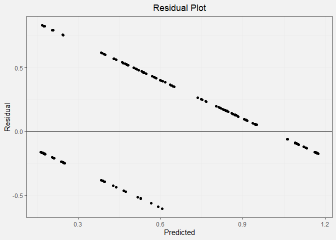
In the residual plot, we expect to see symmetrically distributed points forming a cloud. We also hope to see low residual values and no clear patterns. This is not the case for our data because the output must be a 0 or a 1. This causes the linear regression model to form two distinctive lines on the plot.
Q-Q Plot:
ggplot(mod_results, aes(sample = residual)) +
    geom_qq()+
  geom_qq_line() +
  theme_bw() +
  labs(title="Q-Q Plot", x="Theoretical Quantile", y="Sample Quantile") +
  theme(plot.title = element_text(hjust = 0.5)) +
  theme(plot.background = element_rect(fill = '#f2f2f2', colour = '#f2f2f2')) +
  theme(panel.background = element_rect(fill = '#f2f2f2', colour = '#f2f2f2'))
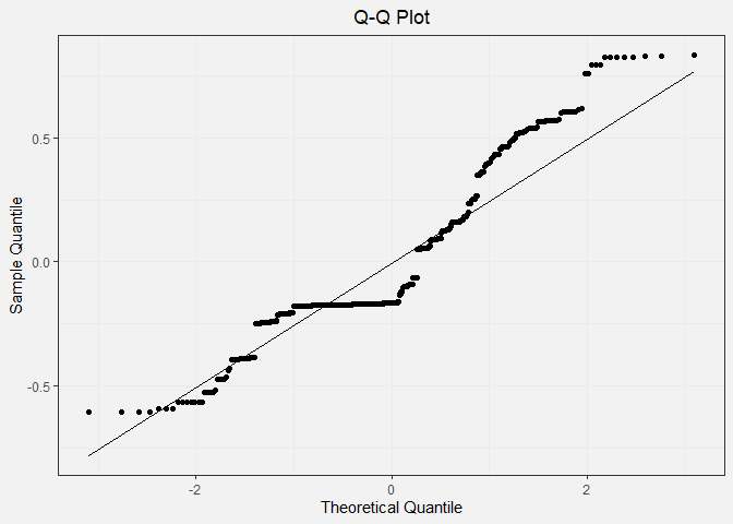
In the Q-Q plot, we expect to see the points in the scatter plot to closely follow the diagonal line. This pattern is clearly not observed.
The mean and standard deviation for our residuals can be calculated as such:
mean_res <- mean(mod_results$residual)
sd_res <- sd(mod_results$residual)
print(c(mean_res, sd_res))
## [1] -2.469760e-17 3.095141e-01
Conclusion
Overall, our assumptions are not met, and a linear regression model is not a good way to model our data.
Random Forest Model
Loading Random Forest Libraries
require(randomForest)
require(caTools)
require(tidyverse)

set.seed(2020)
Loading in Data
We can read in the data using the read_csv() function. The parameters
included in this function are to transform the categorical data into
factor data types for easy analysis later on.
diabetes_data_upload <- read_csv(
  "../data/diabetes_data_upload.csv",
  col_types = cols(
    Gender = col_factor(levels = c("Male", "Female")),
    Polyuria = col_factor(levels = c("Yes", "No")),
    Polydipsia = col_factor(levels = c("Yes", "No")),
    `sudden weight loss` = col_factor(levels = c("Yes", "No")),
    weakness = col_factor(levels = c("Yes", "No")),
    Polyphagia = col_factor(levels = c("Yes", "No")),
    `Genital thrush` = col_factor(levels = c("Yes", "No")),
    `visual blurring` = col_factor(levels = c("Yes", "No")),
    Itching = col_factor(levels = c("Yes", "No")),
    Irritability = col_factor(levels = c("Yes", "No")),
    `delayed healing` = col_factor(levels = c("Yes", "No")),
    `partial paresis` = col_factor(levels = c("Yes", "No")),
    `muscle stiffness` = col_factor(levels = c("Yes", "No")),
    Alopecia = col_factor(levels = c("Yes", "No")),
    Obesity = col_factor(levels = c("Yes", "No")),
    class = col_factor(levels = c("Positive", "Negative"))
  )
)

diabetes_data_upload <- data.frame(diabetes_data_upload)

summary(diabetes_data_upload)
##       Age           Gender    Polyuria  Polydipsia sudden.weight.loss weakness
##  Min.   :16.00   Male  :328   Yes:258   Yes:233    Yes:217            Yes:305
##  1st Qu.:39.00   Female:192   No :262   No :287    No :303            No :215
##  Median :47.50
##  Mean   :48.03
##  3rd Qu.:57.00
##  Max.   :90.00
##  Polyphagia Genital.thrush visual.blurring Itching   Irritability
##  Yes:237    Yes:116        Yes:233         Yes:253   Yes:126
##  No :283    No :404        No :287         No :267   No :394
##
##
##
##
##  delayed.healing partial.paresis muscle.stiffness Alopecia  Obesity
##  Yes:239         Yes:224         Yes:195          Yes:179   Yes: 88
##  No :281         No :296         No :325          No :341   No :432
##
##
##
##
##       class
##  Positive:320
##  Negative:200
##
##
##
##
In the summary of our data, we see that there are more patients with diabetes than without, which calls into question the validity of our model. While dataset is unbalanced, 320 vs 200 is not a very large difference, so our model should still be reasonably accurate.
Splitting Data into a Training and Testing Set
In preparation modeling our data, we can first separate it into a testing and a training set with a split ratio of 0.8. This means that 80% of our overall dataset will be used for training and 20% will be used for testing the model at the end.
sample = sample.split(diabetes_data_upload$class, SplitRatio = .80)
train = subset(diabetes_data_upload, sample == 1)
test  = subset(diabetes_data_upload, sample == 0)

dim(train)
## [1] 416 17
dim(test)
## [1] 104 17
Building the Model
We will build a random forest model using the randomForest() function
and typical default parameter values of 100 trees in the forest.
rf <- randomForest(
  class ~ .,
  data=train,
  ntree = 100,
  importance = TRUE
)
rf
##
## Call:
##  randomForest(formula = class ~ ., data = train, ntree = 100,      importance = TRUE)
##                Type of random forest: classification
##                      Number of trees: 100
## No. of variables tried at each split: 4
##
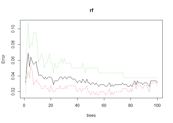
##         OOB estimate of  error rate: 3.12%
## Confusion matrix:
##          Positive Negative class.error
## Positive      249        7  0.02734375
## Negative        6      154  0.03750000
train_accuracy <- (rf$confusion[1,1] + rf$confusion[2,2]) / (dim(train)[1])
After training the random forest model, we see that our model has a training accuracy of 96.9%.
We can plotting the model error vs the number of trees in the forest below and we observe that our model likely does not need the default amount of 100 trees. The error starts to sharply decrease with the first few trees, but then it quickly plateaus.
plot(rf)
Variable Importance
par(bg="#f2f2f2")
varImpPlot(rf, main="Variable Importance Plot", type=1, pch=19)
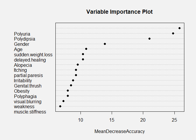
The random forest model is very interesting because it can allow us to
investigate the relative importance of the variables that we use in our
model. In the variable importance plot above, we see that polydipsia,
polyuria, gender, and age are the four most important variables in our
model. This is determined by computing the MeanDecreaseAccuracy. This
quantity is calculated by changing the values in each feature and then
observing how much that change decreases the accuracy of the model. An
interesting conclusion from this plot is that age is very important to
the accuracy of the model. In our density plots above, we concluded that
there was only a slight difference in the mean ages between the patients
that had diabetes and did not have diabetes, and age also was not
statistically significant in the linear model. Therefore, it is likely
that age has a nonlinear relationship with the diabetes status of a
patient or that age in combination with another factor is an important
predictor.
Validating on the Testing Set
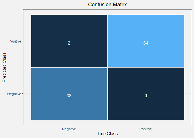
Seeing that the model had good accuracy on the training set and the conclusions from the variable importance plot are reasonable, we can now validate our model on the remaining 20% of the dataset. We use our random forest model to generate predictions for the remaining samples and then compare those with the observed diabetes status of those patients. Finally, we can visualize this with a confusion matrix.
prediction_for_table <- predict(rf,test[,-17])
confusion <- table(observed=test[[17]],predicted=prediction_for_table)
confusion
##           predicted
## observed   Positive Negative
##   Positive       64        0
##   Negative        2       38
true_class <- factor(c('Negative', 'Negative', 'Positive', 'Positive'))
predicted_class <- factor(c('Negative', 'Positive', 'Negative', 'Positive'))
counts      <- c(confusion[2,2], confusion[2,1], confusion[1,2], confusion[1,1])
df <- data.frame(true_class, predicted_class, counts)


ggplot(data =  df, mapping = aes(x = true_class, y = predicted_class)) +
  geom_tile(aes(fill = counts), colour = "white") +
  geom_text(aes(label = sprintf("%1.0f", counts)), vjust = 1, colour="white") +
  scale_fill_gradient() +
  theme_bw() + theme(legend.position = "none") +
  labs(title="Confusion Matrix",x="True Class", y="Predicted Class")+
  theme(plot.title = element_text(hjust = 0.5)) +
  theme(plot.background = element_rect(fill = '#f2f2f2', colour = '#f2f2f2')) +
  theme(panel.background = element_rect(fill = '#f2f2f2', colour = '#f2f2f2'))
test_accuracy <- (confusion[2,2] + confusion[1,1])/sum(confusion)
print(test_accuracy)
## [1] 0.9807692
From our confusion matrix, we can see that the testing accuracy of our model is 98.1%. This value is similar to that of our training accuracy, indicating that our model is not over-fitting to the data. These model accuracy values are very good, and our model has great predictive power. We can do further hyper-parameter tuning to improve our model more, but that is out of the scope of this project.
Conclusion
Overall, the presence of conditions such as polyuria, polydipsia, sudden weight loss, and partial paresis increased the likelihood that a patient has diabetes. The random forest model showed to be a very accurate model for predicting diabetes unlike the linear model. Therefore, the random forest model indicates the polyuria, polydipsia, age, and gender are the useful features for predicting the diagnosis of diabetes.